
There’s a number in quality engineering that’s supposed to tell you whether a measurement system can be trusted: the Gauge R&R study. It’s a good tool. But if you’ve ever run one on a balancing machine and felt like the result didn’t quite match what the machine was actually doing, that instinct is correct. The standard formula wasn’t built for what balancing measures.
What GRR Was Built For
Traditional Gauge R&R assumes a specific kind of measurement: a single characteristic, on a single axis, checked against two limits. A shaft diameter has an upper spec and a lower spec, and a well-behaved measurement system produces a bell curve centered somewhere between them. The classic formula, 5.15σ/Tol, is a comparison of two ranges: how wide your measurement spread is, versus how wide your tolerance band is. It’s a clean fit, because the thing being measured is genuinely one-dimensional.
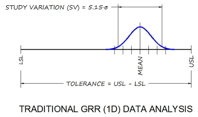
Unbalance Isn’t One-Dimensional
Unbalance is a vector. It has a magnitude and an angle, and it’s measured relative to a rotational center rather than a fixed axis. There’s also no lower limit, only an upper one: a maximum allowable radius. That radius is set by the application rather than by the machine, and it varies widely across part types, from turbine rotors to turbocharger wheels (See Applications). So you have two-dimensional data being evaluated against a tolerance zone that is a circle, not a band.
Where that radius gets set is a separate question, and tightening it is not automatically an improvement.
Run 5.15σ/Tol on that anyway and you are implicitly doing two things you probably didn’t intend. You throw away all of the angular information, and you compare a linear range to a tolerance that was never linear in the first place. The formula still returns a number. It just isn’t measuring what you think it is.
There’s a subtler issue hiding in there. When an unbalance distribution is centered near the origin, which is exactly what you want from a well-performing machine, converting that 2D data to magnitude-only values distorts its statistical shape. A symmetric, normal distribution in two dimensions becomes skewed and non-normal once it is flattened into a single number. In other words, the better the machine performs, the more the magnitude-only math misrepresents it.
The Fix: Evaluate It as a Circle
If the tolerance is a circle, the study variation should be too. That is the idea behind MU95. Instead of measuring spread along an axis, you find the radius of the circle that contains 95% of your measured points, then compare that radius directly to the tolerance radius.
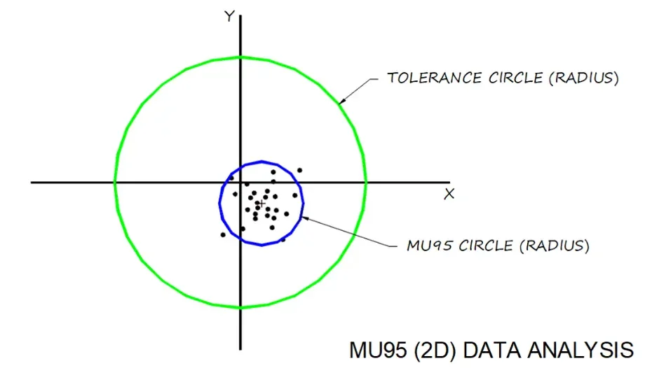
MU95/Tol is the two-dimensional equivalent of 5.15σ/Tol, and it holds up because both sides of the ratio describe the same kind of geometry. You are comparing a radius to a radius, rather than a range to something that was never a range.
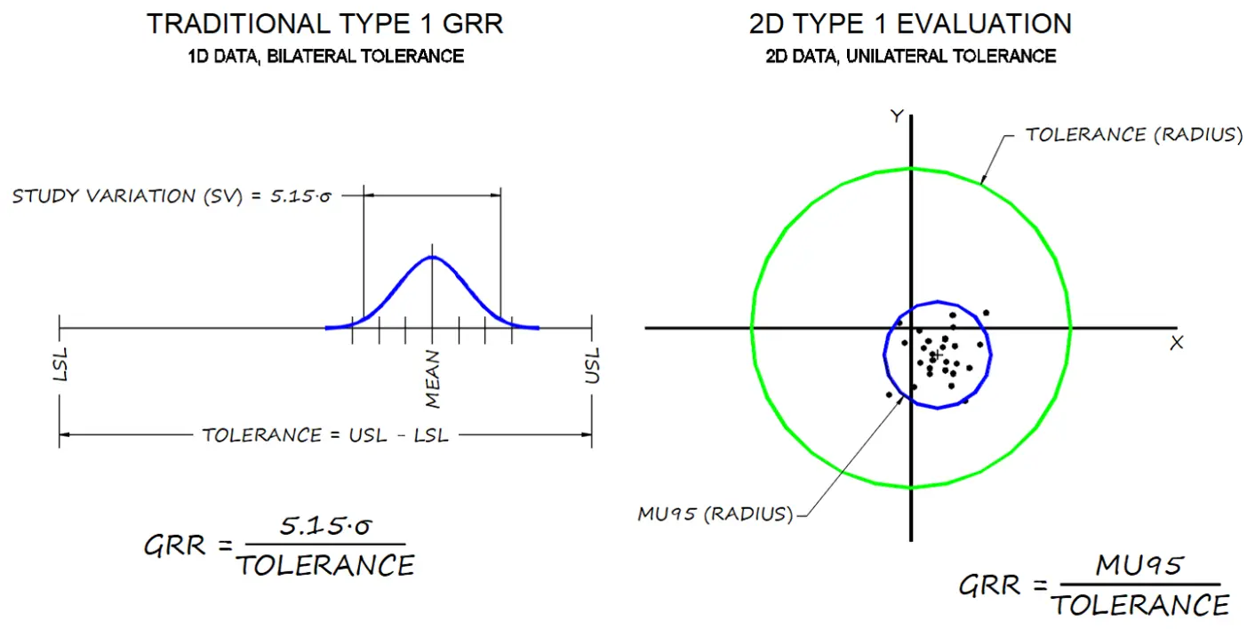
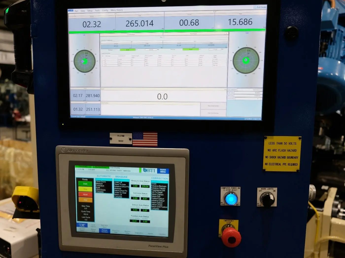
On modern equipment this isn’t a manual spreadsheet exercise. Balancers can run these studies themselves, executing the protocol and reporting spin-to-spin repeatability and Gage R&R results directly, with operating modes that separate machine repeatability from tooling and part-handling effects (See Automated Capability Testing).
One practical note: MU95 needs the underlying point data, not a summary figure. Machines that log every reading and export it as .csv will import straight into Minitab or Excel, where fitting a 95% radius is a short calculation. Getting the export format sorted out before the study is easier than reconstructing it afterward (See Statistics and Production Data).
When You Can’t Switch Entirely
Sometimes a magnitude-only dataset is already built into your process, and rebuilding it isn’t realistic. There’s a reasonable middle ground: keep the 5.15σ numerator, but divide by 2×Tol instead of Tol. Doubling the denominator reframes the comparison as range versus range again, which keeps the units consistent even though it doesn’t account for the angular data. It’s a workable approximation, and it applies to conventional Type 2 and 3 studies as well.
If the obstacle is access to a controlled setup rather than the math itself, running the study in a dedicated measurement and testing lab is a reasonable way to get a baseline before committing to a method (See In-House Measurement & Testing Services).
The Takeaway
Balancing systems measure vectors, not scalars, so evaluating them with a purely linear tool will always be an approximation at best. MU95/Tol is the more accurate approach, and the 2×Tol adjustment is a reasonable stand-in when a full transition isn’t practical. Either way, the math should match the geometry of what is actually being measured.
This is one of a few places where a standard quality metric doesn’t transfer cleanly to balancing. Cpk runs into a similar mismatch when a machine inspects every part rather than a sample.
One caveat is worth keeping in view. Any capability study is only as trustworthy as its reference. A study run against a certified master rotor with NIST traceable weights measures something real. One run against a previous reading measures agreement with itself (See Calibration & Certification Services).